Quickstart for Deep Reinforcement Learning in rlberry
In this tutorial, we will focus on Deep Reinforcement Learning with the Advantage Actor-Critic algorithm.
Imports
from rlberry.envs import gym_make
from rlberry.manager import plot_writer_data, ExperimentManager, evaluate_agents
from rlberry.agents.stable_baselines import StableBaselinesAgent
from stable_baselines3 import PPO
Reminder of the RL setting
We will consider a MDP \(M = (\mathcal{S}, \mathcal{A}, p, r, \gamma)\) with:
\(\mathcal{S}\) the state space,
\(\mathcal{A}\) the action space,
\(p(x^\prime \mid x, a)\) the transition probability,
\(r(x, a, x^\prime)\) the reward of the transition \((x, a, x^\prime)\),
\(\gamma \in [0,1)\) is the discount factor.
A policy \(\pi\) is a mapping from the state space \(\mathcal{S}\) to the probability of selecting each action. The action value function of a policy is the overall expected reward from a state action. \(Q^\pi(s, a) = \mathbb{E}_{\tau \sim \pi}\big[R(\tau) \mid s_0=s, a_0=a\big]\) where \(\tau\) is an episode \((s_0, a_0, r_0, s_1, a_1, r_1, s_2, ..., s_T, a_T, r_T)\) with the actions drawn from \(\pi(s)\); \(R(\tau)\) is the random variable defined as the cumulative sum of the discounted reward.
The goal is to maximize the cumulative sum of discount rewards:
Gymnasium Environment
In this tutorial we are going to use the Gymnasium library (previously OpenAI’s Gym). This library provides a large number of environments to test RL algorithm.
We will focus only on the Acrobot-v1 environment, although you can experimenting with other environments such as CartPole-v1 or MountainCar-v0. The following table presents some basic components of the three environments, such as the dimensions of their observation and action spaces and the rewards occurring at each step.
Env Info |
CartPole-v1 |
Acrobot-v1 |
MountainCar-v0 |
|---|---|---|---|
Observation Space |
Box(4) |
Box(6) |
Box(2) |
Action Space |
Discrete(2) |
Discrete(3) |
Discrete(3) |
Rewards |
1 per step |
-1 if not terminal else 0 |
-1 per step |
Running A2C on Acrobot-v1
⚠ warning: depending on the seed, you may get different results. ⚠
In the next example we use default parameters PPO and we use rlberry to train and evaluate the Stable Baselines PPO agent.
"""
The ExperimentManager class is a compact way of experimenting with a deepRL agent.
"""
default_xp = ExperimentManager(
StableBaselinesAgent, # The Agent class.
(gym_make, dict(id="Acrobot-v1")), # The Environment to solve.
fit_budget=1e5, # The number of interactions
# between the agent and the
# environment during training.
init_kwargs=dict(algo_cls=PPO), # Init value for StableBaselinesAgent
eval_kwargs=dict(eval_horizon=500), # The number of interactions
# between the agent and the
# environment during evaluations.
n_fit=3, # The number of agents to train.
# Usually, it is good to do more
# than 1 because the training is
# stochastic.
agent_name="PPO default", # The agent's name.
)
print("Training ...")
default_xp.fit() # Trains the agent on fit_budget steps!
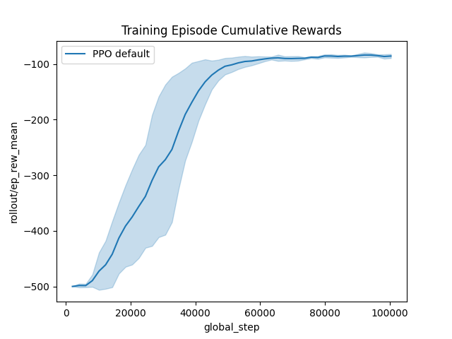
# Plot the training data:
_ = plot_writer_data(
[default_xp],
tag="rollout/ep_rew_mean",
title="Training Episode Cumulative Rewards",
show=True,
)
Training ...
[INFO] 09:31: Running ExperimentManager fit() for PPO default with n_fit = 3 and max_workers = None.
[INFO] 09:31: [PPO default[worker: 0]] | max_global_step = 4096 | time/iterations = 1 | rollout/ep_rew_mean = -500.0 | rollout/ep_len_mean = 500.0 | time/fps = 791 | time/time_elapsed = 2 | time/total_timesteps = 2048 | train/learning_rate = 0.0003 |
[INFO] 09:31: [PPO default[worker: 1]] | max_global_step = 4096 | time/iterations = 1 | rollout/ep_rew_mean = -500.0 | rollout/ep_len_mean = 500.0 | time/fps = 741 | time/time_elapsed = 2 | time/total_timesteps = 2048 | train/learning_rate = 0.0003 |
[INFO] 09:31: [PPO default[worker: 2]] | max_global_step = 4096 | time/iterations = 1 | rollout/ep_rew_mean = -500.0 | rollout/ep_len_mean = 500.0 | time/fps = 751 | time/time_elapsed = 2 | time/total_timesteps = 2048 | train/learning_rate = 0.0003 |
[INFO] 09:32: [PPO default[worker: 0]] | max_global_step = 6144 | time/iterations = 2 | rollout/ep_rew_mean = -500.0 | rollout/ep_len_mean = 500.0 | time/fps = 617 | time/time_elapsed = 6 | time/total_timesteps = 4096 | train/learning_rate = 0.0003 | train/entropy_loss = -1.0967000976204873 | train/policy_gradient_loss = -0.0017652213326073251 | train/value_loss = 139.4249062538147 | train/approx_kl = 0.004285778850317001 | train/clip_fraction = 0.0044921875 | train/loss = 16.845857620239258 | train/explained_variance = -0.0011605024337768555 | train/n_updates = 10 | train/clip_range = 0.2 |
...
...
...
[INFO] 09:35: [PPO default[worker: 1]] | max_global_step = 100352 | time/iterations = 48 | rollout/ep_rew_mean = -89.81 | rollout/ep_len_mean = 90.8 | time/fps = 486 | time/time_elapsed = 202 | time/total_timesteps = 98304 | train/learning_rate = 0.0003 | train/entropy_loss = -0.19921453138813378 | train/policy_gradient_loss = -0.002730156043253373 | train/value_loss = 21.20977843105793 | train/approx_kl = 0.0014179411809891462 | train/clip_fraction = 0.017626953125 | train/loss = 9.601455688476562 | train/explained_variance = 0.8966712430119514 | train/n_updates = 470 | train/clip_range = 0.2 |
[INFO] 09:35: [PPO default[worker: 0]] | max_global_step = 100352 | time/iterations = 48 | rollout/ep_rew_mean = -83.22 | rollout/ep_len_mean = 84.22 | time/fps = 486 | time/time_elapsed = 202 | time/total_timesteps = 98304 | train/learning_rate = 0.0003 | train/entropy_loss = -0.14615743807516993 | train/policy_gradient_loss = -0.002418491238495335 | train/value_loss = 22.7100858271122 | train/approx_kl = 0.0006727844011038542 | train/clip_fraction = 0.010546875 | train/loss = 8.74121379852295 | train/explained_variance = 0.8884317129850388 | train/n_updates = 470 | train/clip_range = 0.2 |
[INFO] 09:35: ... trained!
[INFO] 09:35: Saved ExperimentManager(PPO default) using pickle.
[INFO] 09:35: The ExperimentManager was saved in : 'rlberry_data/temp/manager_data/PPO default_2024-04-24_09-31-51_be15b329/manager_obj.pickle'
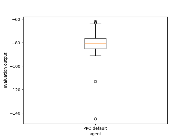
print("Evaluating ...")
_ = evaluate_agents(
    [default_xp], n_simulations=50, show=True
)  # Evaluate the trained agent on
# 10 simulations of 500 steps each.
Evaluating ...
[INFO] 09:36: Evaluating PPO default...
[INFO] Evaluation:..................................................  Evaluation finished
Let’s try to change the hyperparameters and see if it change the previous result.
⚠ warning: The aim of this section is to show that hyperparameters have an effect on agent training, and to demonstrate that it is possible to modify them.
For pedagogical purposes, since the default hyperparameters are effective on these simple environments, we’ll compare the default agent with an agent tuned with the wrong hyperparameters, which decreases the results. Obviously, in practical cases, the aim is to find hyperparameters that improve results… not decrease them. ⚠
tuned_xp = ExperimentManager(
    StableBaselinesAgent,  # The Agent class.
    (gym_make, dict(id="Acrobot-v1")),  # The Environment to solve.
    init_kwargs=dict(  # Where to put the agent's hyperparameters
        algo_cls=PPO,
        # gradient descent steps.
        # descent steps.
        ent_coef=0.10,  # How much to force exploration.
        normalize_advantage=False,  # normalize the advantage
        gae_lambda=0.90,  # Factor for trade-off of bias vs variance for Generalized Advantage Estimator
        n_epochs=20,  # Number of epoch when optimizing the surrogate loss
        n_steps=64,  # The number of steps to run for the environment per update
        learning_rate=1e-3,
        batch_size=32,
    ),
    fit_budget=1e5,  # The number of interactions
    # between the agent and the
    # environment during training.
    eval_kwargs=dict(eval_horizon=500),  # The number of interactions
    # between the agent and the
    # environment during evaluations.
    n_fit=3,  # The number of agents to train.
    # Usually, it is good to do more
    # than 1 because the training is
    # stochastic.
    agent_name="PPO incorrectly tuned",  # The agent's name.
)


print("Training ...")
tuned_xp.fit()  # Trains the agent on fit_budget steps!


# Plot the training data:
_ = plot_writer_data(
    [default_xp, tuned_xp],
    tag="rollout/ep_rew_mean",
    title="Training Episode Cumulative Rewards",
    show=True,
)
Training ...
[INFO] 09:37: Running ExperimentManager fit() for PPO incorrectly tuned with n_fit = 3 and max_workers = None.
[INFO] 09:37: [PPO incorrectly tuned[worker: 1]] | max_global_step = 832 | time/iterations = 12 | time/fps = 260 | time/time_elapsed = 2 | time/total_timesteps = 768 | train/learning_rate = 0.001 | train/entropy_loss = -0.9725531369447709 | train/policy_gradient_loss = 5.175539326667786 | train/value_loss = 17.705344581604002 | train/approx_kl = 0.028903376311063766 | train/clip_fraction = 0.33828125 | train/loss = 8.651824951171875 | train/explained_variance = 0.03754150867462158 | train/n_updates = 220 | train/clip_range = 0.2 | rollout/ep_rew_mean = -251.0 | rollout/ep_len_mean = 252.0 |
[INFO] 09:37: [PPO incorrectly tuned[worker: 2]] | max_global_step = 832 | time/iterations = 12 | time/fps = 260 | time/time_elapsed = 2 | time/total_timesteps = 768 | train/learning_rate = 0.001 | train/entropy_loss = -1.0311604633927345 | train/policy_gradient_loss = 5.122353088855744 | train/value_loss = 18.54480469226837 | train/approx_kl = 0.02180374786257744 | train/clip_fraction = 0.359375 | train/loss = 9.690193176269531 | train/explained_variance = -0.00020706653594970703 | train/n_updates = 220 | train/clip_range = 0.2 | rollout/ep_rew_mean = -500.0 | rollout/ep_len_mean = 500.0 |
...
...
...
[INFO] 09:45: ... trained!
[INFO] 09:45: Saved ExperimentManager(PPO incorrectly tuned) using pickle.
[INFO] 09:45: The ExperimentManager was saved in : 'rlberry_data/temp/manager_data/PPO incorrectly tuned_2024-04-24_09-37-32_33d1646b/manager_obj.pickle'
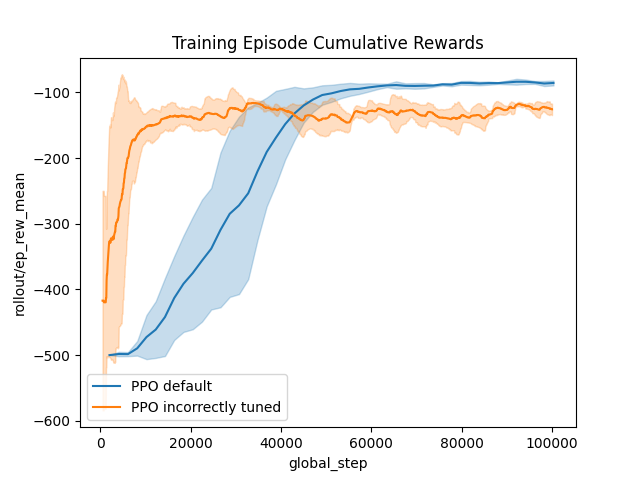
Here, we can see that modifying the hyperparameters has change the learning process (for the worse): it learns faster, but the final result is lower…
☀ : For more information on plots and visualization, you can check here (in construction)
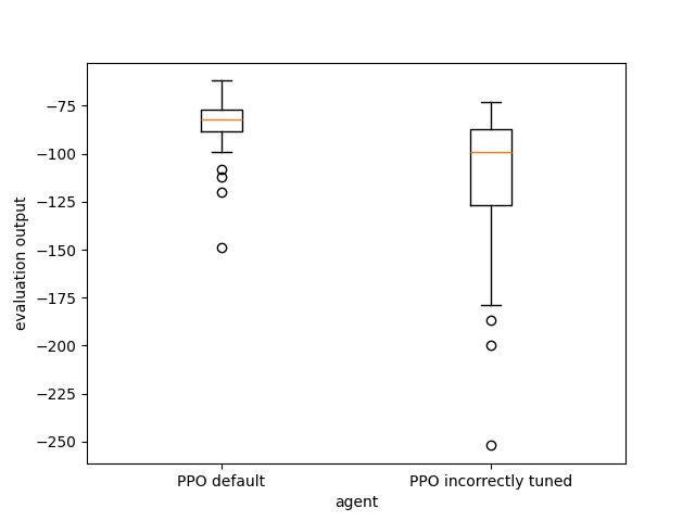
print("Evaluating ...")

# Evaluating and comparing the agents :
_ = evaluate_agents([default_xp, tuned_xp], n_simulations=50, show=True)
Evaluating ...
[INFO] 09:47: Evaluating PPO default...
[INFO] Evaluation:..................................................  Evaluation finished
[INFO] 09:47: Evaluating PPO incorrectly tuned...
[INFO] Evaluation:..................................................  Evaluation finished