rlberry.manager.plot_writer_data
- rlberry.manager.plot_writer_data(data_source, tag, xtag=None, smooth=False, smoothing_bandwidth=None, id_agent=None, ax=None, error_representation='ci', n_boot=500, level=0.9, sub_sample=True, show=True, preprocess_func=None, title=None, savefig_fname=None, linestyles=False)[source]
Given a list of ExperimentManager or a folder, plot data (corresponding to info) obtained in each episode. The dictionary returned by agents’ .fit() method must contain a key equal to info.
If there are several simulations, a confidence interval is plotted. In all cases a smoothing is performed
- Parameters:
- data_source
ExperimentManager, or list ofExperimentManageror str or list of str If ExperimentManager or list of ExperimentManager, load data from it (the agents must be fitted).
If str, the string must be the string path of a directory, each
subdirectory of this directory must contain pickle files. load the data from the directory of the latest experiment in date. This str should be equal to the value of the output_dir parameter in
ExperimentManager.If list of str, each string must be a directory containing pickle files
load the data from these pickle files.
Note: the agent’s save function must save its writer at the key _writer. This is the default for rlberry agents.
- tagstr
Tag of data to plot on y-axis.
- xtagstr or None, default=None
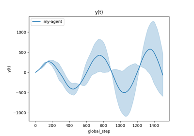
Tag of data to plot on x-axis. If None, use ‘global_step’. Another often-used x-axis is the time elapsed dw_time_elapsed, in which case smooth needs to be set to True or there must be only one run.
- smoothboolean, default=False
Whether to smooth the curve with a Nadaraya-Watson Kernel smoothing. Remark that this also allow for an xtag which is not synchronized on all the simulations (e.g. time for instance).
- smoothing_bandwidth: float or array of floats or None
How to choose the bandwidth parameter. If float, then smoothing_bandwidth is used directly as a bandwidth. If is an array, a parameter search using smoothing_bandwidth is used. If None, a parameter search from a range of 20 possible values choosen by heuristics is performed.
- id_agentint or None, default=None
id of the agent to plot, if not None plot only the results for the agent whose id is id_agent.
- ax: matplotlib axis or None, default=None
Matplotlib axis on which we plot. If None, create one. Can be used to customize the plot.
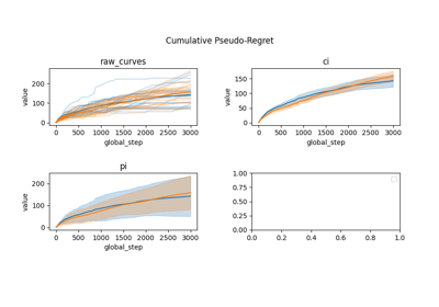
- error_representation: str in {“cb”, “raw_curves”, “ci”, “pi”}
How to represent multiple simulations. The “ci” and “pi” do not take into account the need for simultaneous inference, it is then harder to draw conclusion from them than with “cb” and “pb” but they are the most widely used.
“cb” is a confidence band on the mean curve using functional data analysis (band in which the mean curve is with probability larger than 1-level).
“raw curves” is a plot of the raw curves.
“pi” is a plot of a non-simultaneous prediction interval with gaussian model around the mean smoothed curve (e.g. we do curve plus/minus gaussian quantile times std).
“ci” is a confidence interval with gaussian model around the mean smoothed curve (e.g. we do curve plus/minus gaussian quantile times std divided by sqrt of number of seeds).
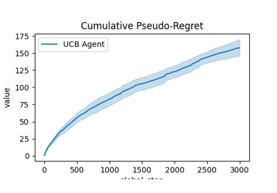
- n_boot: int, default=500,
Number of bootstrap evaluations used for confidence interval estimation. Only used if error_representation = “ci”.
- level: float, default=0.95,
Level of the confidence interval. Only used if error_representation = “ci”
- sub_sample, boolean, default = True,
If True, use up to 1000 points for one given seed of one agent to reduce computational cost.
- show: bool, default=True
If True, calls plt.show().
- preprocess_func: Callable, default=None
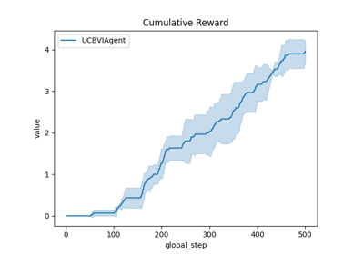
Function to apply to ‘tag’ column before plot. For instance, if tag=episode_rewards, setting preprocess_func=np.cumsum will plot cumulative rewards. If None, do nothing. Warning: this function should return an array of the same size as the input.
- title: str (Optional)
Optional title to plot. If None, set to tag.
- savefig_fname: str (Optional)
Name of the figure in which the plot is saved with figure.savefig. If None, the figure is not saved.
- linestyles: boolean, default=False
Whether to use different linestyles for each curve.
- Returns
- ——-
- Pandas DataFrame with processed data.
- data_source
Examples
>>> from rlberry_research.agents.torch import A2CAgent, DQNAgent
>>> from rlberry.manager import ExperimentManager, plot_writer_data
>>> from rlberry.envs import gym_make
>>>
>>> if __name__=="__main__":
>>>     managers = [ ExperimentManager(
>>>         agent_class,
>>>         (gym_make, dict(id="CartPole-v1")),
>>>         fit_budget=4e4,
>>>         eval_kwargs=dict(eval_horizon=500),
>>>         n_fit=1,
>>>         parallelization="process",
>>>         mp_context="spawn",
>>>         seed=42,
>>>          ) for agent_class in [A2CAgent, DQNAgent]]
>>>     for manager in managers:
>>>         manager.fit()
>>>     # We have only one seed (n_fit=1) hence the curves are automatically smoothed
>>>     data = plot_writer_data(managers, "episode_rewards")
Examples using rlberry.manager.plot_writer_data

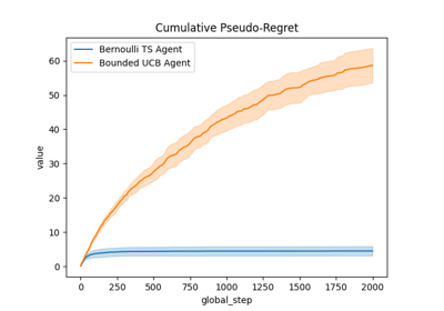
Comparison of Thompson sampling and UCB on Bernoulli and Gaussian bandits
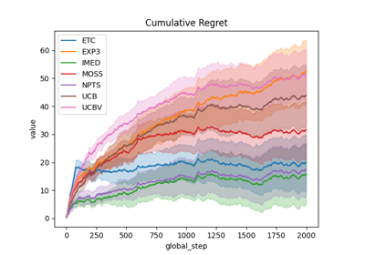
Comparison subplots of various index based bandits algorithms